Matching flight to OTM data and Predicting Thermal Landscapes
predict_thermal_landscapes.RmdOverview
In this vignette, our goal is to illustrate the process behind the
final step of the throne workflow; the prediction of
spatio-temporally complete thermal landscapes. To achieve this,
throne uses two functions: match_data and
predict_thermal_landscpe. The first allows the user to
match the thermal dynamics of a given tile within their site (i.e., a
unique x and y UTM coordinate combination) as
measured across multiple flights with those of an operative
temperature model (OTM). The second, uses this
matches data set and combines it with information from date & OTM
specific cubic spline models (obtained using the
gen_otm_splines function) to predict the temperature of
each tile in the area of interest at any moment in time while the OTMs
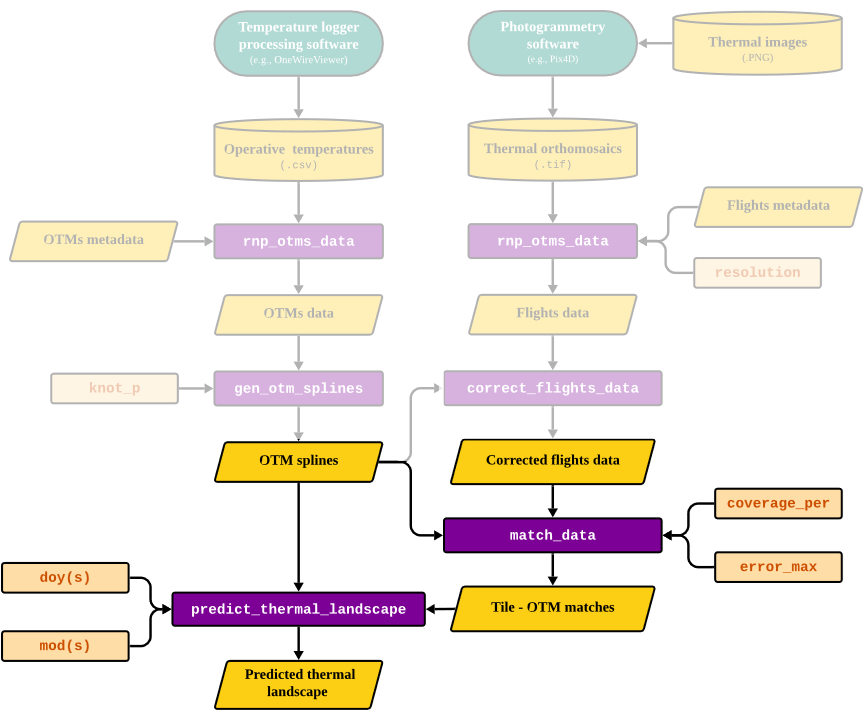
were deployed in the field. In the context of the overall workflow of
the package, this is the section that is covered in this vignette:
The match_data function
The match_data function matches the thermal dynamics of
specific tiles collected across multiple flights to the thermal dynamics
of an operative temperature model
(OTM). This will typically be the longest step
in the throne pipeline but, if done correctly, the
user will only need to run it once. Next, we discuss the function’s
inputs, processes and output
Inputs
Te match_data function takes in the following
inputs:
A flight data set obtained using the
rnp_flights_data. We strongly recommend that this data undergoes correction using thecorrect_flights_datafunction in order to ensure that both flights and OTM data are on an operative temperature scale. However, the function will allow the user to use uncorrected data if they so choose.An
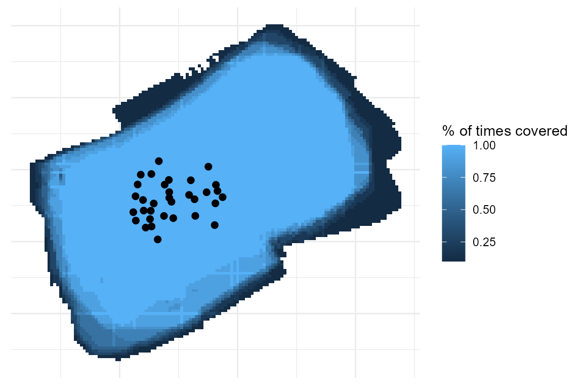
otm_splinesnestedtibbleobtained using thegen_otm_splinesfunction.coverage_per, a numeric value between 0 - 1 indicating the minimum coverage that a tile should have across all flights provided in order to be included in the matching process. The need for this input can be easily visualized by overlapping the area covered by multiple flights in the provided exampleflights_data(see below). Due to the unique conditions during each flight, the area covered is variable, specially when focusing around the edges of the area of interest. To circumvent this, we recommend that the area covered by each flight should be much larger than the area of interest. With the example data, our goal was to encompass the area where OTMs were deployed in the ground (black dots), and as seen below, we achieved that. As a general guideline, we recommend settingcoverage_per >= 0.9, the value the function will default to ifcoverage_peris not specified. Nonetheless, the function output will also provide acoveragecolumn for each tile to further inform the users.
-
error_max, the maximum error between temperature measurements of a tile and the OTM that best represents it, which we elaborate on below.
Processes
To match tiles with OTMs that best describe their thermal dynamics,
the match_data function goes through the following general
steps:
It calculates the coverage across all flights for every single tile covered and selects only those tiles that have been covered as much or more as the
coverage_perargument specifies.For each tile, calculate the average absolute error between the temperature measurements of that tile during each flight and the temperature measurements made by every OTM at the exact same time each flight took place.
Select the OTM that minimizes the error between the tile’s and the OTMs measurements. In the figure below we illustrate the logic of this approach. The black dots indicate the temperature measurements associated with a given tile (note that these measurements are corrected using the
correct_flights_datafunction) across all flights conducted in the days of the year (doy) 236, 237 and 238. The red and blue lines indicate the temperatures predicted by the spline model of 2 OTMs for those samedoy. Between these two, thematch_datafunction would chooseOTM25to better represent the dynamics of that tile as the average difference between each of the tile’s temperature measurements and those estimated by the cubic spline model forOTM25is smaller than forOTM05.
## Generating OTM & doy-specific spline models...## | | | 0% | |= | 1% | |= | 2% | |== | 2% | |== | 3% | |=== | 4% | |=== | 5% | |==== | 5% | |==== | 6% | |===== | 7% | |===== | 8% | |====== | 8% | |====== | 9% | |======= | 10% | |======= | 11% | |======== | 11% | |========= | 12% | |========= | 13% | |========== | 14% | |========== | 15% | |=========== | 15% | |=========== | 16% | |============ | 17% | |============ | 18% | |============= | 18% | |============= | 19% | |============== | 20% | |============== | 21% | |=============== | 21% | |=============== | 22% | |================ | 23% | |================= | 24% | |================== | 25% | |================== | 26% | |=================== | 27% | |==================== | 28% | |==================== | 29% | |===================== | 30% | |===================== | 31% | |====================== | 31% | |====================== | 32% | |======================= | 33% | |======================== | 34% | |========================= | 35% | |========================= | 36% | |========================== | 37% | |=========================== | 38% | |=========================== | 39% | |============================ | 40% | |============================= | 41% | |============================= | 42% | |============================== | 43% | |============================== | 44% | |=============================== | 44% | |================================ | 45% | |================================ | 46% | |================================= | 47% | |================================== | 48% | |================================== | 49% | |=================================== | 50% | |==================================== | 51% | |==================================== | 52% | |===================================== | 53% | |====================================== | 54% | |====================================== | 55% | |======================================= | 56% | |======================================== | 56% | |======================================== | 57% | |========================================= | 58% | |========================================= | 59% | |========================================== | 60% | |=========================================== | 61% | |=========================================== | 62% | |============================================ | 63% | |============================================= | 64% | |============================================= | 65% | |============================================== | 66% | |=============================================== | 67% | |================================================ | 68% | |================================================ | 69% | |================================================= | 69% | |================================================= | 70% | |================================================== | 71% | |================================================== | 72% | |=================================================== | 73% | |==================================================== | 74% | |==================================================== | 75% | |===================================================== | 76% | |====================================================== | 77% | |======================================================= | 78% | |======================================================= | 79% | |======================================================== | 79% | |======================================================== | 80% | |========================================================= | 81% | |========================================================= | 82% | |========================================================== | 82% | |========================================================== | 83% | |=========================================================== | 84% | |=========================================================== | 85% | |============================================================ | 85% | |============================================================ | 86% | |============================================================= | 87% | |============================================================= | 88% | |============================================================== | 89% | |=============================================================== | 89% | |=============================================================== | 90% | |================================================================ | 91% | |================================================================ | 92% | |================================================================= | 92% | |================================================================= | 93% | |================================================================== | 94% | |================================================================== | 95% | |=================================================================== | 95% | |=================================================================== | 96% | |==================================================================== | 97% | |==================================================================== | 98% | |===================================================================== | 98% | |===================================================================== | 99% | |======================================================================| 100%## Spline generation complete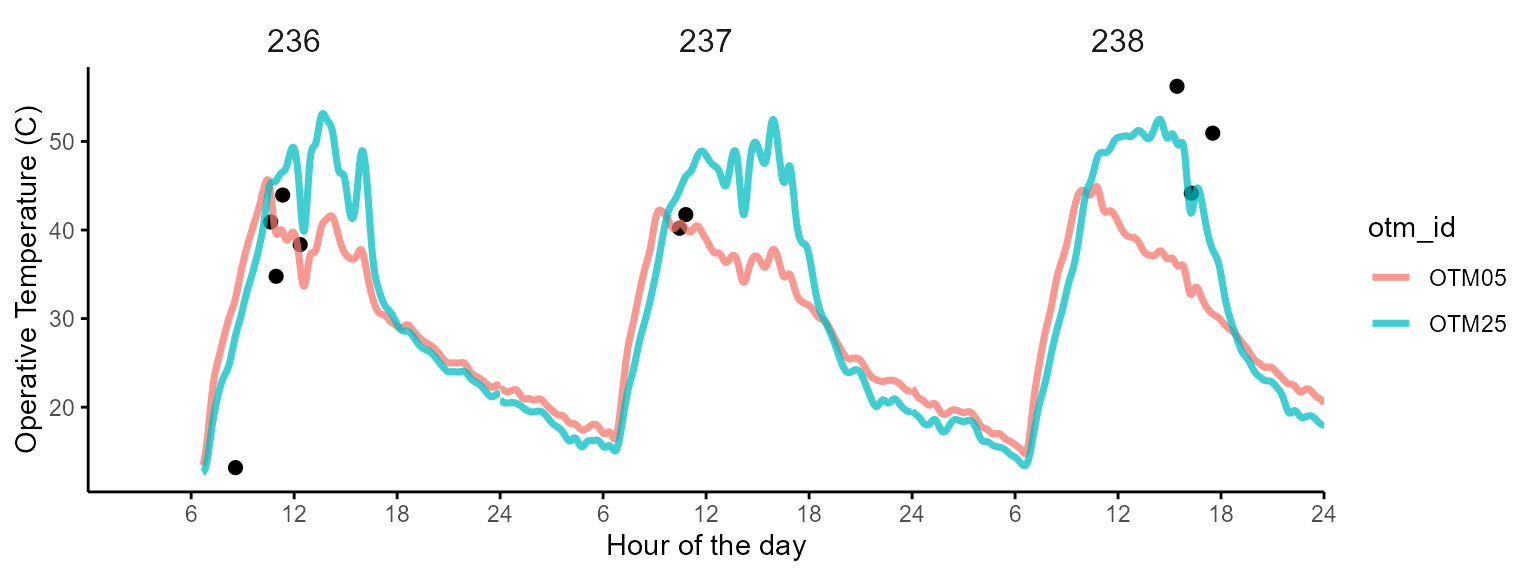
NOTE: The distance between the tile and the OTM is NOT weighted for during this step. This is because an OTM that is not necessarily the closest to that tile might actually be able to represent its thermal dynamics much better than one that is closer. For example, a tile that contains a tree might be better represented by an OTM that is deployed inside of a tree at 100 m than one that is on a different facing slope only 2 m away. This approach extends even to a the same tile where an OTM is deployed. Imagine a tile that is mostly facing south but that has a small bush on it. If an OTM is placed precisely inside that bush, its thermal dynamics might not be representative of the average dynamics of that tile and an OTM placed elsewhere might actually represent that tile better. In the figure below we show the results of matching our example data set, where only in 5 cases the same OTM that was on a tile best described its thermal dynamics.
- If the minimum error is above a certain threshold indicated by the
error_maxparameter do not assign any OTM to a tile. In the figure below we show the results of implementing this step with the areas marked in dark blue indicating tiles for which no OTM could describe it without exceeding the threshold imposed byerror_max(error_max = 5in this case). It is also important to note that these “problematic” tiles are far from the area of interest for this study (where the OTMs, indicated by black dots, where deployed) and that in this area the error is minimized.
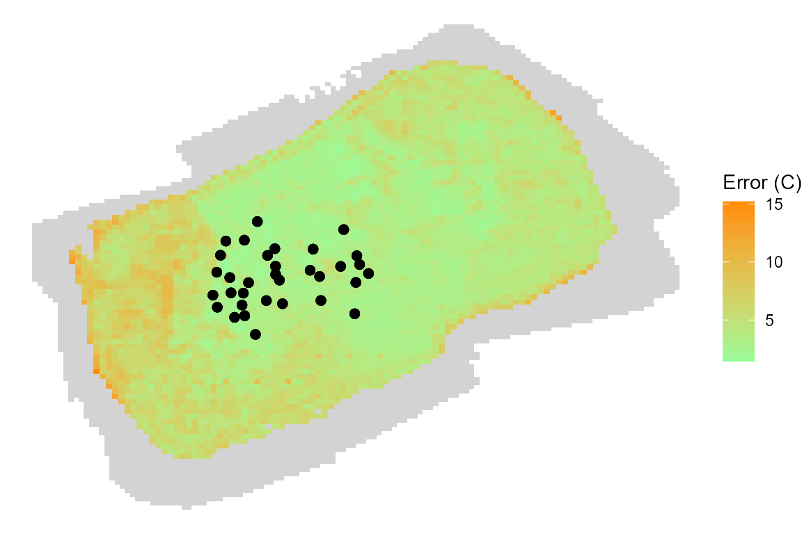
NOTE: The figure above shows all tiles that were covered by at least 1 flights but that were not covered in at least 90% of flights shaded in light gray. As seen above, the high-coverage area is much smaller than the total area covered in flights.
As seen above, error rarely exceeds 10 C. This is a good
indication that the OTMs are well suited to describe the thermal
dynamics of the area of interest. Below is the distribution of error to
further illustrate this point.
## Warning: Removed 1 row containing non-finite outside the scale range
## (`stat_density()`).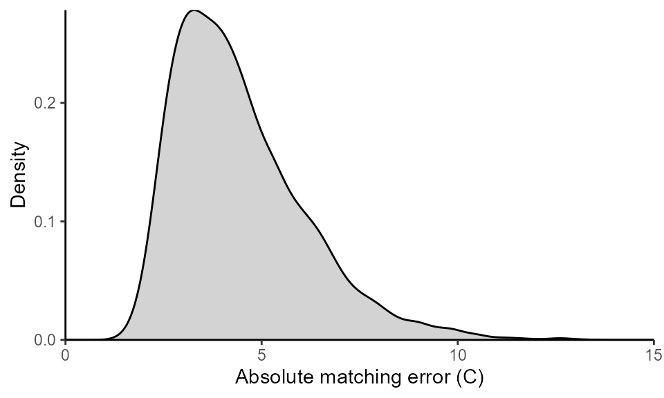
The resulting matches has the otm_id column
indicating the OTM that best describes a given tile (i.e., a combination
of x and y coordinates) as well as a columns
for the matching error and the coverage across
flights for the user to inspect if desired. In rows where
error > error_max the otm_id will be
specified as NA. Below we show how the function would be
run and its output:
# mock code to show how match_data would need to be ran
matches <- match_data(flights_data = flights_data_corrected,
                      otm_splines = otms_splines,
                      error_max = 10, # allowing a maximum error of 10 C as an example
coverage_per = 0.9) # setting coverage across flights to 90%## x y coverage error otm_id
## 1594 275257.2 4416493 0.9411765 13.107961 OTM37
## 1626 275257.2 4416494 0.9117647 11.903082 OTM37
## 1657 275257.2 4416496 0.9117647 10.479966 OTM11
## 2308 275258.4 4416488 0.9117647 8.957312 OTM02
## 2339 275258.4 4416490 0.9411765 9.262035 OTM02
## 2371 275258.4 4416491 0.9705882 11.695899 OTM26NOTE: The
matchesdata set presented above was generated considering witherror_max = 100that can be accessed by callingmatches. Both data sets were generated by settingcoverage_per = 0.9, the default setting.
From this matches data we gather some interesting
findings. Including that:
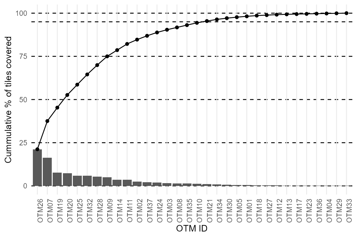
- Very few OTMs are needed to explain the majority of the sites
thermal dynamics. In the example data set, only
5out of the33deployed OTMs deployed were needed to explain more than over 50% of the thermal variability of the site.
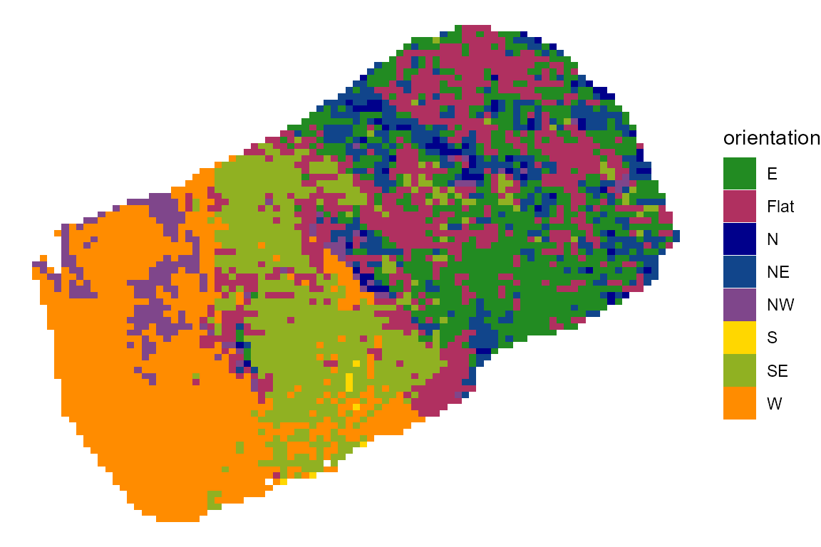
- The matching mechanism will automatically match tiles with a given
orientation to OTMs deployed in a tile with the same orientation. As
seen below and considering that the site is plotted in a N-S
orientation, we can, for example, see that OTMs facing
Wbest described tiles that were on a western slope and so on.
Predicting thermal landscapes
The final step in the workflow of the throne package is
to predict thermal landscapes. To do this, the package includes the
function predict_thermal_landscape. Next, we will discuss
the function’s inputs, processes and outputs.
Inputs
An
otm_splinesnestedtibbleobtained through thegenerate_otm_splines.A
matchesdata set associating tiles in a study area with OTMs that best describe their thermal dynamics obtained using thematch_datafunction discussed above.The day of the year or
doy(single or multiple) for which a prediction should be generated.The minute of the day or
mod(single or multiple) in thedoyspecified for which a prediction should be generated.
Processes
Then, predict_thermal_landscape will go through the
following general steps:
Filter the
otm_splinesfor splines characterizing OTMs that are also present in thematchesobject, and, among these, select only models describing the dynamics of that OTM on thedoy(single or multiple) specified as an argument of the function.Predict the operative temperature at the specified
mod(single or multiple) anddoyfor all OTMs.Merge the operative temperature prediction with the
matchesto obtain a predicted operative temperature for every tile considered.
Output
The final output of the function will be a data.frame of
predicted operative temperature values. Since all the necessary
calculations have been carried out beforehand (i.e., generating the
spline models, performing the matching between tiles and OTMs etc.)
predict_thermal_landscape is relatively fast and allows the
user to predict the entire thermal landscape of their site at
any moment while OTMs were deployed. For example, below is how
one would obtain a complete thermal landscape prediction every hour of
the day for the doy = 237 (i.e., August 24th):
# obtain prediction using system.time to show duration
system.time(prediction_237 <- predict_thermal_landscape(matches = throne::matches,
                                                        otm_splines = otms_splines,
                                                        doy = 237,
                                                        mod = seq(0,1440, by = 60))) # every hour)
## user system elapsed
## 0.64 0.02 0.66
head(prediction_237)## otm_id x y coverage doy mod pred_op_temp
## 1 OTM01 275317.2 4416522 1 237 0 21.50141
## 2 OTM01 275317.2 4416522 1 237 60 21.27824
## 3 OTM01 275317.2 4416522 1 237 120 20.07036
## 4 OTM01 275317.2 4416522 1 237 180 19.05241
## 5 OTM01 275317.2 4416522 1 237 240 17.58155
## 6 OTM01 275317.2 4416522 1 237 300 17.03824NOTE: The
predict_thermal_landscapefunction will not be able to predict thermal landscapes if the specified time falls outside of the range when OTMs were logging temperatures. To that end, the function will also provide a warning indicating what % of predictions were removed due to falling outside of the range when the OTMs were recording.
We can plot this prediction using regular ggplot:
prediction_237 |>
  filter(mod %in% seq(6*60,21*60,by = 60)) |>
  filter(!is.na(mod)) |>
  ggplot(aes(x = x, y = y, fill = pred_op_temp)) +
  geom_raster() +
  scale_fill_viridis(option = "magma") +
  facet_wrap(~mod/60) +
  theme_void() +
  theme(
    legend.position = "top",
    strip.text = element_text(size = 12)
    ) +
  guides(fill = guide_colorbar(title = "Predicted Operative Temperature (C)"))
The predict_thermal_landscape function has unlimited power
to provide complete thermal landscape predictions at an unprecedented
level of detail. To showcase the entire throne pipeline in
action, next we present a case study exemplifying how to implement the
method.