Reading and processing OTM data and Generating OTM spline models
rnp_otms_data_gen_otm_splines.RmdOverview
The goal of this vignette is to illustrate the process behind the
rnp_otms_data (read and
process OTMs data) and gen_otm_splines
(generate OTM spline
models) functions of the throne package.
The first function allows the user to read one or multiple raw
.csv (see “Collecting
OTM data vignette”) with temperature measurements recorded by a
temperature logger inside of an operative temperature
model (OTM) to a data frame in R.
The second function takes this processed OTM data and generates an OTM
& day of year (doy) specific cubic spline model that
describes the thermal dynamics of each unique OTM each day. These spline
models will later be used to both correct
the flights data and to ultimately predict
thermal landscapes. Below, we highlight the section of the package’s
workflow that is covered in this vignette:
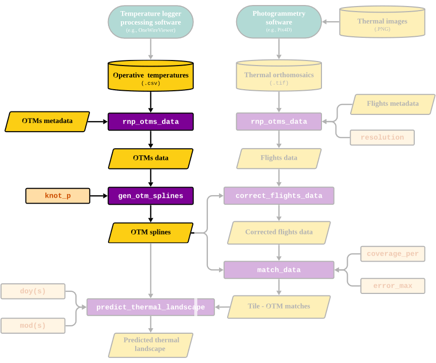
Next, we will discuss each function in detail.
Reading and processing OTM data
The rnp_otms_data function reads a database of
.csv files, manipulates and ultimately combines them into a
large data.frame in R. Below we detail the
function’s inputs, processes and output
Inputs
The rnp_otms_data function takes the following
inputs:
-
path, the directory where one or multiple.csvfiles are stored. Each of these.csvfiles is assumed to have at least:
A column for operative temperature measurements. Since different temperature logger processing software structure the outputs differently in the resulting
.csvfile,thronerequires the user to specify the column where the OTM measurements can be found in theop_temp_colargument of the function. We used OneWire Viewer which returns the operative temperature in the3rd column.A column for dates. As with the operative temperature values,
thronealso requires the user to specify thedate_colin their.csvfiles. OneWireViewer returns the date in the first column inMM/DD/YY HH:MM:SS AM/PMformat. By default dates and times will be extracted from this column but other software return date and time in separate columns. If that is the case, the user can specify thetime_colas an argument of the function.
TIP: Users of
throneshould become very familiar with the formatting of the.csvfiles containing OTM data. In some software options, the resulting.csvfile will contain several rows of metadata that might lead to an incorrect reading of the file (see example below). While thernp_otms_datawill provide warnings we also recommend the users to specify how many rows should be skipped when reading each file file via therows_skipargument. Specifying therows_skipargument correctly is crucial for the rest of the package’s functions to work properly down the line. For more information, see the function’s documentation here
- An OTM
metadatadata.frameortibblecontaining information related to each specific OTM (identified by a uniqueotm_id). The user can include any metadata for the OTM but we require that anotm_idcolumn is present and we strongly recommend that the metadata also contains columns for thelatitudeandlongitudeat which the OTM was deployed. In the example metadata shipped withthronewe also incorporate information on themicrohabitat,orientationandelevationat which the OTM was deployed.
head(otms_metadata)## # A tibble: 6 × 6
## otm_id microhabitat orientation latitude longitude elevation
## <chr> <chr> <chr> <dbl> <dbl> <dbl>
## 1 OTM01 outcrop N 39.9 -120. 1312.
## 2 OTM21 outcrop NW 39.9 -120. 1312.
## 3 OTM07 outcrop E 39.9 -120. 1312.
## 4 OTM16 outcrop SE 39.9 -120. 1313.
## 5 OTM17 outcrop Flat 39.9 -120. 1311.
## 6 OTM28 rock Flat 39.9 -120. 1313.Processes
To transform the raw .csv data into a
data.frame the rnp_otm_data function will go
through the following general steps:
- Read each
.csvfile while skipping as many rows as specified within therows_skipargument. - Select the columns for time and operative temperature as specified
by the
date_col(and/ortime_col) andop_temp_colarguments. - Re-project
latitudeandlongitudecoordinates toxandyUTM coordinates to enable compatibility with the rest of the package’s functionality using tools from theterrapackage - Using tools from the
lubridatepackage, extract theyear, day of the year (doy)and minute of the day (mod) at which each operative temperature measurement (op_temp) was made.
NOTE: Working
doyandmodallows the user to work with numeric colums. This simplifies the management of the data, as dates and times have unique data formats in theRenvironment that are often difficult to handle and may lead unintended errors. Nonetheless, these formats can be transformed back into more interpretable temporal scales for visualization purposes, by using theas.Datefunction to transformdoy(also known as Julian date) back into a YYYY-MM-DD format and dividing by 60 formodto get hours.
- Merge the processed data for each OTM with its corresponding metadata and, if more than one file is specified, bind the outputs together.
Output
The final output is a data.frame like this:
head(otms_data)## otm_id year doy mod op_temp microhabitat orientation latitude longitude
## 1 OTM01 2023 236 367 13.5 outcrop N 39.86873 -119.627
## 2 OTM01 2023 236 369 13.5 outcrop N 39.86873 -119.627
## 3 OTM01 2023 236 371 13.5 outcrop N 39.86873 -119.627
## 4 OTM01 2023 236 373 13.5 outcrop N 39.86873 -119.627
## 5 OTM01 2023 236 375 13.5 outcrop N 39.86873 -119.627
## 6 OTM01 2023 236 377 13.5 outcrop N 39.86873 -119.627
## elevation x y
## 1 1311.73 275314.9 4416490
## 2 1311.73 275314.9 4416490
## 3 1311.73 275314.9 4416490
## 4 1311.73 275314.9 4416490
## 5 1311.73 275314.9 4416490
## 6 1311.73 275314.9 4416490Each row will corresponds to a unique operative temperature
(op_temp) measurement by a given otm_id in a
given year, doy and mod. Our
example data set contains measurements of 33 OTMs over 4 days recording
at a rate of 720 observations / day (30 observations / h, 0.5
observations / min).
Generating OTM cubic spline models
The next step in the throne workflow will be to fit a
cubic smoothing spline model to each OTM each
doy during it’s deployment in the field. This model will
capture the thermal dynamics of the OTM in a given doy
enabling a temporally continuous prediction of operative temperature
from discrete measurements. To achieve this, throne
includes the gen_otm_splines function, which takes as input
the output generated via rnp_otms_data. The function will
then calculate OTM and doy specific splines and return a
nested tibble with an OTM identifier column, associated
metadata, together with a nested column
containing the model generated via the native R function
smooth.spline. Below we show how to use the
gen_otm_splines function:
otm_splines_ex <- gen_otm_splines(otm_data = otms_data, knot_p = 0.02) %>%
  dplyr::select(-c("microhabitat", "orientation", "elevation"))
otm_splines_ex## # A tibble: 132 × 8
## otm_id year doy latitude longitude x y spline
## <chr> <dbl> <dbl> <dbl> <dbl> <dbl> <dbl> <list>
## 1 OTM01 2023 236 39.9 -120. 275315. 4416490. <smth.spl>
## 2 OTM01 2023 237 39.9 -120. 275315. 4416490. <smth.spl>
## 3 OTM01 2023 238 39.9 -120. 275315. 4416490. <smth.spl>
## 4 OTM01 2023 239 39.9 -120. 275315. 4416490. <lgl [1]>
## 5 OTM02 2023 236 39.9 -120. 275285. 4416482. <smth.spl>
## 6 OTM02 2023 237 39.9 -120. 275285. 4416482. <smth.spl>
## 7 OTM02 2023 238 39.9 -120. 275285. 4416482. <smth.spl>
## 8 OTM02 2023 239 39.9 -120. 275285. 4416482. <lgl [1]>
## 9 OTM03 2023 236 39.9 -120. 275291. 4416498. <smth.spl>
## 10 OTM03 2023 237 39.9 -120. 275291. 4416498. <smth.spl>
## # ℹ 122 more rowsWhy splines?: Using a smoothing function as opposed to modelling OTM thermal fluctuations using biophysical principles offers, in this case, a more flexible approach. Smoothing minimizes noise from short-term, stochastic shifts in operative temperature while capturing fluctuations caused by conditions unique to each day (e.g., sustained changes in cloud cover or wind) that may be ecologically relevant. This approach eliminates the need to collect additional metadata during OTM deployment (e.g., aspect or shade cover) and removes the assumption that within-day thermal fluctuations follow a fixed sinusoidal curve in order to inform the resulting models. Nonetheless, as the level of smoothing may be important in certain systems and may influence the ability of
throneto match OTMs with orthomosaic tiles, thegen_otm_splinesfunction incorporates the parameterknot_pwhich allows users to determine their desired level of smoothness
Choosing the appropriate knot_p value
A critical point for the gen_otm_splines function to
work correctly is determining the appropriate value for the
knot_p argument. This argument determines the percentage of
observations recorded by an OTM in a given day that are used to
determine the number of knots of the smoothing spline model. The number
of knots will ultimately determine the degrees of freedom of the model
as \(df = degree + k\) and \(degree = 3\) for cubic splines (see here
for further details). The number of degrees of freedom will then
determine the “wiggliness” of the resulting model, i.e. the number of
times the resulting curve will change direction. As an example, below we
plot different spline models for the same data using different
knot_p parameter values.
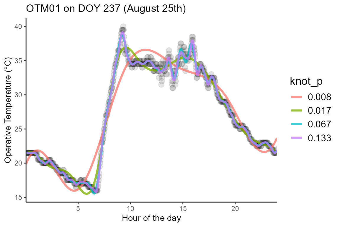
The first factor to consider is the frequency at which the
OTM itself is recording. We can extrapolate how many knots/day
(or knots/h) we would get based on the frequency of recordings and the
knot_p value according to the formula:
\[ Knot/h = Recordings/h \cdot knot_p\]
For instance, the OTMs we use as an example in this package were
programmed to record a temperature measurement every 2 minutes, leading
to a total of 30 observations / hour. Assuming a
knot_p = 0.1 that would indicate that our model has 3 knots
/ h. We recommend setting knot_p to a higher value if the
frequency of observations is low, but the decision ultimately comes to
the user of the methodology. Feel free to reach out to the package
maintainer for recommendations.
The second issue that determines the value of knot_p is
the study organism. Generally, OTMs will equilibrate to the
environmental temperature much faster than the organism they represent
with this difference in equilibration time being positively correlated
to the mass of the organism due to thermal inertia. We recommend
understanding the thermal properties of the organism of interest when
choosing the appropriate knot_p value as we did in our
pilot study.
Having shown how to read and process both flights and OTM data the next step will be to correct the flights data to transform surface temperature to operative temperature temperature measurements.