Reading and processing flight data

Overview

The goal of this vignette is to illustrate the process behind the rnp_flights_data (read and process flights data) function of the throne package. This function enables processing of raw .tif files obtained by combining images collected during a drone flight (see the Flying drones and obtaining thermal orthomosaics vignette) into a data frame structure easily manageable in R. This data frame will later be related to operative temperature model (OTM) data to finally predict thermal landscapes. Below, we highlight the section of the package’s workflow that is covered in this vignette:

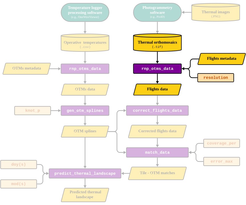
Next, we present how the rnp_flights_data function works by discussing it’s inputs, processes and output

Inputs

The rnp_flights_data takes in 3 inputs:

The path to the directory where all thermal orthomosaics (i.e., .tif files) for flights are stored.
A data.frame with metadata for each flight. This data.frame must contain specific columns indicating the flight_id, the date when the flight took place and the times at which the flight started and ended. For more specific information please check the function’s documentation here. Below is an example data set included with throne illustrating how the metadata should be structured:

##    flight_id      date time_start time_end
## 1    VAL2_01 8/24/2023       8:35     8:39
## 6    VAL2_06 8/24/2023      10:38    10:42
## 7    VAL2_07 8/24/2023      10:57    11:01
## 8    VAL2_08 8/24/2023      11:20    11:24
## 11   VAL2_11 8/24/2023      12:21    12:25
## 12   VAL2_12 8/25/2023      10:27    10:31
## 13   VAL2_13 8/25/2023      10:49    10:53
## 25   VAL2_25 8/26/2023      15:26    15:30
## 27   VAL2_27 8/26/2023      16:16    16:20
## 30   VAL2_30 8/26/2023      17:31    17:35

The spatial resolution to which the .tif files should be summarized to in \(m^2\). This parameter will control the spatial resolution of the final output and should be chosen according to the spatial scale of the study organism. The lower boundry for spatial resolution is set to \(0.5 m^2\) and while there is no upper boundry we recommend users to set resolution to a value that is not larger than the area they are studying.

Processes

To transform the original .tif files, the rnp_flights_data goes through the following steps for all .tif files specified:

Read each specified .tif file as a as a raster object using the rast function from the terra package.
Re-scale the resolution of the raster object to the desired spatial resolution using terra’s aggregate function.
Transform the raster object into a data.frame.
Add metadata information, including the year, day of the year (doy) and minute of the day when the flight started (mod_start) and ended (mod_end).

NOTE: Working doy and mod allows the user to work with numeric colums. This simplifies the management of the data, as dates and times have unique data formats in the R environment that are often difficult to handle and may lead unintended errors. Nonetheless, these formats can be transformed back into more interpretable temporal scales for visualization purposes, by using the as.Date function to transform doy (also known as Julian date) back into a YYYY-MM-DD format and dividing by 60 for mod to get hours.

Output

The final output of rnp_flights_data is a data.frame with the following columns:

x and y: UTM coordinates.
year, doy, mod_start, mod_end: The year, day of the year, minute of the day when the flight started and ended respectively.
surf_temp: Surface IR-measured temperature (°C).

Thus, each row on the data.frame will correspond to a unique surf_temp measurement on a particular tile (a unique x and y combination) within a specific flight. The number of rows will in turn depend on 1) the number of flights processed and 2) the desired spatial resolution.

Below is an example data set showing how the output of rnp_flights_data should look like:

##         x       y surf_temp year doy mod_start mod_end
## 75 275330 4416550  25.82156 2023 236       515     519
## 76 275331 4416550  25.08232 2023 236       515     519
## 77 275332 4416550  23.77567 2023 236       515     519
## 78 275333 4416550  24.48907 2023 236       515     519
## 79 275334 4416550  19.89712 2023 236       515     519
## 80 275335 4416550  10.46925 2023 236       515     519

These data can already be processed to visualize and quantify the thermal characteristics of a study site. Below we illustrate how to visualize this data using ggplot2 and 4 of the 10 fully processed flights (with a spatial resolution of \(1m^2\)) we include in the flights_data example data set that is included with throne. Panel titles indicate the hour in which the flight took place.

flights_data |>
  filter(mod_start %in% c(515, 680, 926, 1051)) |>
  filter(surf_temp > 12) |>
  mutate(hour = round(mod_start/60)) |>
  mutate(hour = paste(hour,":00 h", sep = "")) |>
  ggplot(aes(x = x, y = y, fill = surf_temp)) +
  geom_raster() +
  scale_fill_viridis("Surface temperature (°C)", option = "magma") +
  facet_wrap(~ fct_reorder(hour, mod_start)) +
  xlab("Longitude") + ylab("Latitude") +
  theme_void() +
  theme(strip.text = element_text(size = 12),
        legend.position = "top")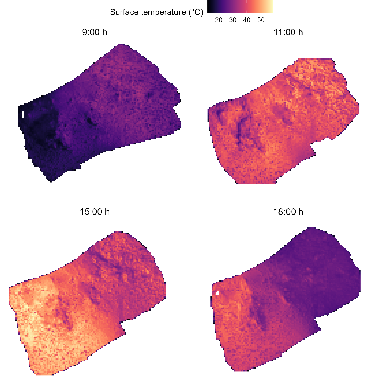

Choosing the appropriate spatial resolution

The rnp_flights_data function allows the user to specify the spatial resolution to which the .tif files should be summarized to. This parameter controls the spatial resolution of the final output and should be chosen according to the spatial scale of the study organism. 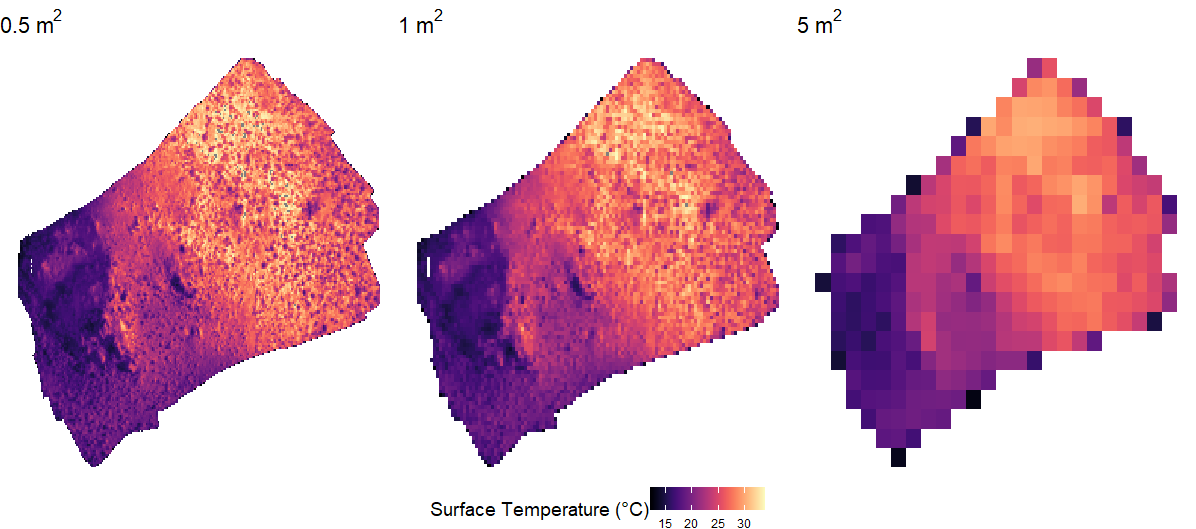We leave it up to the user to determine the appropriate spatial resolution for their system but we consider it important to highlight that a greater resolution will result in a longer processing time in all subsequent steps. To choose the appropriate resolution for their data, we recommend that users run rnp_flights_data at multiple spatial resolutions and visualize the output. Below is a plot illustrating one of the flights we include in throne as an example processed at 0.5, 1 and 5 \(m^2\) of spatial resolution:

Next, we will present how the throne package can read and process OTM data and generate OTM and date specific spline models.

BONUS: Extending the use of `throne`.

While `throne was designed with drone imagery in mind, users of the package can use any geo-referenced spatial raster that is encoded as a .tif file as a source. A potential avenue to extend the use of throne is to use satellite thermal imagery as that provided in the VIIRS, MODIS or Copernicus datasets instead of data from drone flights. Satellite rasters can be treated similarly to drone flights, though each cell will have a much coarser spatial resolution. While this approach is possible, users of throne will face a new logistical challenge in the deployment of OTMs. The recommendations provided in the “Collect OTM data” vignette would need to be adapted to a much larger study area. Users would need to deploy OTMs over a large geographical area making sure that representative microhabitats as well as any latitudinal, elevational or other environmental gradients are captured by OTMs. This would allow users to model operative thermal landscapes at much greater spatial scales at the expense of spatial resolution.